Nonlinear shrinkage estimators

Nonlinear shrinkage estimators correspond to covariance estimators based on the eigendecomposition of the sample matrix:

F = eigen(X)
# ... (transformation of eigenvalues)
F.U*(d̃ .* F.U') # d̃ is a vector of transformed eigenvalues

Currently, there are two flavors of analytical nonlinear shrinkage:

• AnalyticalNonlinearShrinkage is recommended in cases where the covariance matrix can be stored as a dense matrix

• for cases where the covariance matrix is too large to handle in dense form, WoodburyEstimator models the covariance matrix as

  Σ = σ²I + U * Λ * U'

where σ is a scalar, I is the identity matrix, U is a low-rank semi-orthogonal matrix, and Λ is diagonal. One can readily compute with this representation via the Woodbury matrix identity and the WoodburyMatrices package. This formulation approximates the covariance matrix as if all but a few (largest) eigenvalues are equal to σ². A truncated singular value decomposition of the data matrix is performed and the corresponding eigenvalues are shrunk by optimal methods for a wide variety of loss functions:

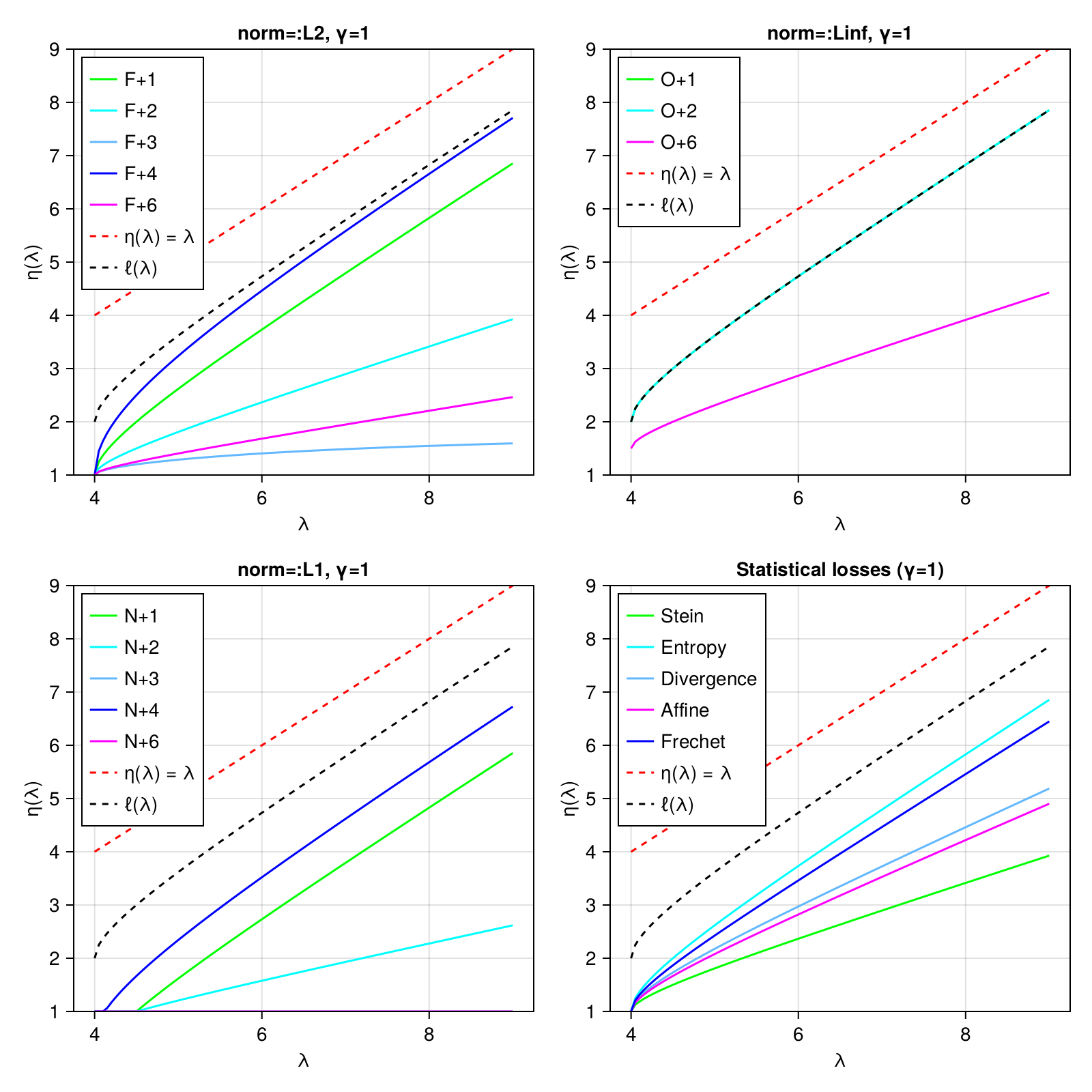
• NormLossCov allows you to specify that you want to minimize some notion of loss against the "true" covariance matrix
• StatLossCov allows you to optimize for certain specific statistical outcomes, e.g., optimizing the accuracy of Mahalanobis distances.

The eigenvalue shrinkage function is plotted for all choices below (γ = p/n, the ratio of the dimensionality to the number of observations):

For complete details, see:

Donoho, D.L., Gavish, M. and Johnstone, I.M., 2018. Optimal shrinkage of eigenvalues in the spiked covariance model. Annals of statistics, 46(4), p.1742.